▷Remove duplicate Excel files: all techniques 🥇

It is not always easy to spot duplicates in a table, especially when it is large. But Excel has many functions to find them, show them, hide them, count them and delete them if necessary.

While it is normal that some of your tables have duplicate data in a particular column - if you are in the trade, luckily you have the right to sell the same product reference on Friday and then on the following Tuesday and Thursday. ! -, it is just as normal to want, at one time or another, to keep only a list of unique data, or to accumulate for these duplicates, or even to perform these two tasks at the same time.

A simple sort on the right column of an Excel table is already enough to identify the same or similar values, whether they are text labels or dates, for example. But Excel was born in 1985, over the versions, it too has accumulated! Today it offers many functions, sometimes redundant or with subtle features, and which can be found in different menus, to help you treat these duplicates as you wish: highlight them, hide them, combine them or calculate the average, or even delete them.

The layout and names of the options differ a bit between versions of Excel for Windows, Mac, and the web, but they operate identically.

How to spot duplicates in one or more columns in Excel?

There are several ways to spot all duplicate values in one or more columns at a glance, without actually removing them.

Click in any cell of your table and, to select all the data in it, press the key combination Ctrl + A on PC or Cmd + A on Mac. Whether or not the first header row (Student, Subject) is part of the selection or not is irrelevant for the function you are going to launch here. Be aware, however, that by pressing again Ctrl + A, the selection would extend to these column titles (if these headers are not already selected), and that a new pressure on Ctrl + A would select the entire sheet.

Remove duplicate Excel files: all techniques

You could also select only one column to only be interested in duplicates in this column: click on the first value (for example on Peter in our example) and press the three keys Ctrl + Shift + Down Arrow, on PC or Mac or in Excel for the Web. You can also click, at the top, on the A de la colonne A.
In the tab Home, click on Conditional Formatting> Cell Highlighting Rules> Duplicate Values.

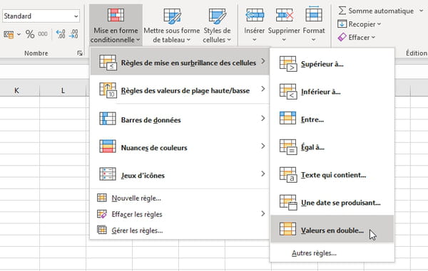
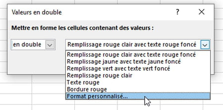
From the first drop-down list, select two fold (the other possible criterion is: unique), and in the second list, choose a cell formatting, for example Light red fill or specify another by clicking on Custom size…

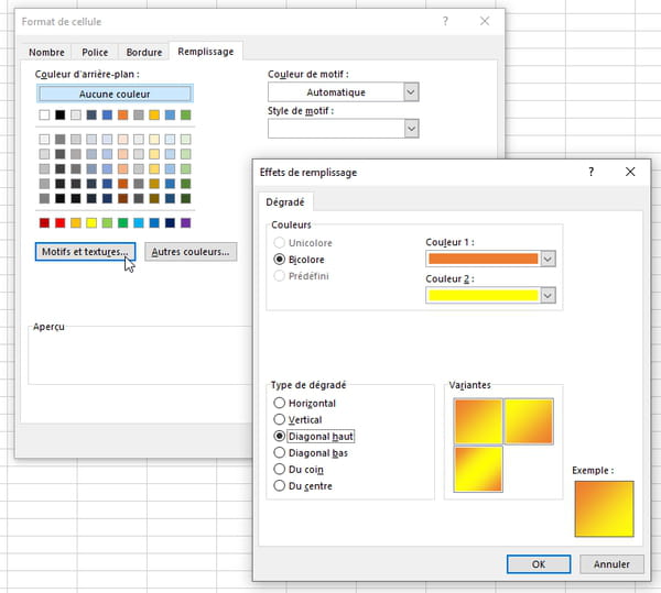
If you have chosen a custom format, the Cell Format lets you choose the formatting of duplicates using the tabs Number, Font, Border et Filling. Click for example on the button Patterns and textures, you can pick two colors from the palette to create a gradient.

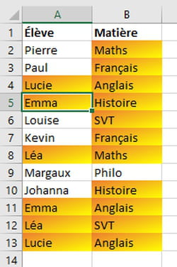
Press several times OK to validate your choices, duplicate cells are formatted as you specified for easier identification.

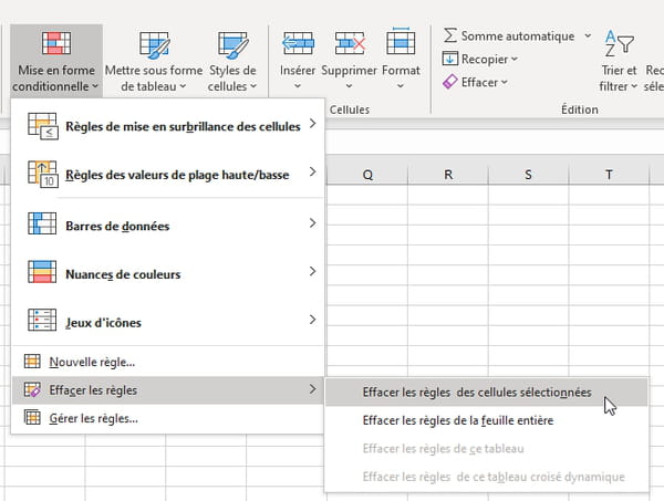
This formatting does not overwrite the old formatting of your cells, it will disappear when you select your table (Ctrl + A ou Cmd + A) and that, in the tab Home, you will launch Conditional Formatting> Clear Rules from Selected Cells. To avoid having to select the whole table, you can also click on Erase the rulers from the entire sheet.

If a value, for example Emma, appears twice in the Student column, Excel marks that value twice as Emma. We specify this because in other functions that we will see later, Excel leaves the first occurrence of Emma intact, but acts only on the following ones, the duplicates.
Even if several columns are selected (as in our example), this Excel function searches for duplicates in each column, independently of the others. Excel therefore does not search the table for all the rows where the pair Emma + History appears, it formats Emma if the first name appears several times in the Student column, and formats History if this caption appears several times in the Subject column. You could also run the command on the first column, then on the second, you would obtain the same results as by launching it straight away on the two columns of the table.
Excel does not take into account the case (capitals): toto, Toto, ToTo and TotO are mentioned as duplicates.
The spreadsheet does not take into account the format either: if three cells store the date 11/11/2021, all will be mentioned as duplicates even if, due to their display format, the first displays 11-Nov, the second 11 / 11 and the third 11/11/20.

How to filter data to show duplicates in Excel?

Filters are very useful for displaying only certain rows in a table. Excel hides rows that don't match your criteria but doesn't remove any data - if you're using an Excel-compatible spreadsheet, you're sure to be offered a filter function. With filters you can, for example, display in a list of products only those whose brand is Sony - which is the same as finding all duplicates of Sony. And just as easily create multicriteria filtering on several columns, such as: Brand = Sony and Category = Television.

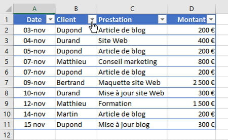
Excel filters are recognizable by the small drop-down arrow that appears to the right of each column header, to sort or filter your data on criteria that you will specify. It is essential that your columns each start with a header (a column title).

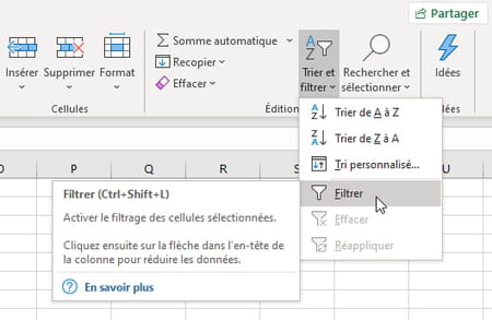
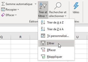
To activate the filters, a first method consists in clicking on a non empty cell of your range of cells and, in the tab Home, to click on Sort and filter, then below on Filter. The keyboard shortcut is Ctrl+Maj+L on macOS and Windows (this icon Filter is also available under the tab Data). Small drop-down arrows appear on the first row containing the headings.

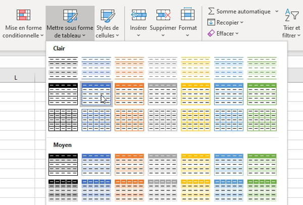
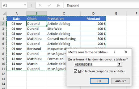
Another possible method to activate filters, more specific to Excel and which offers you more possibilities (you will see a use of this later to calculate the sum of duplicates): create a "table" from your data. Start by clicking on one of your data. Under the tab Home, now click on Format as a table, select a formatting among those proposed ...

… Excel selects the whole table and marks whether or not it has headers. If your columns don't have one, it adds some by inserting a row above it, and calls them Column 1, Column 2, etc. But it is preferable to name your columns yourself (Date, Customer, Service, etc.). Click on OK, the table is formatted and the filters are automatically activated.

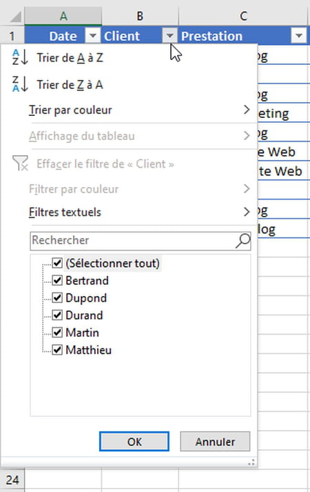
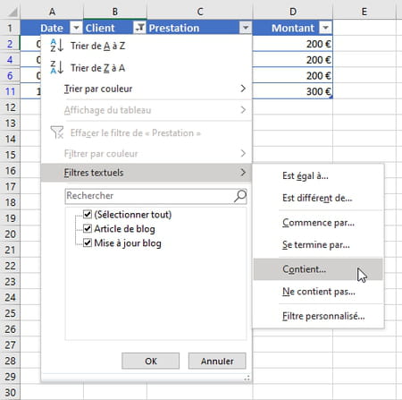
Whichever method you have enabled filters, click a drop down arrow a column title to discover sorting and filtering options. The presentation, although a little different on the Mac, offers the same richness.

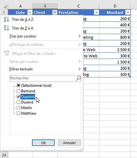
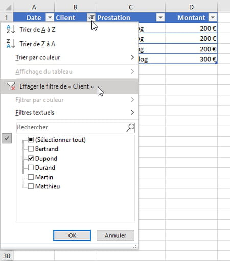
If you only want to see, for example, the lines corresponding to the Dupond customer, the fastest way is to first uncheck the box (Select all) - which will therefore deselect everything -, then to check only the box Dupond (Excel considers Dupond and dupond to be the same).

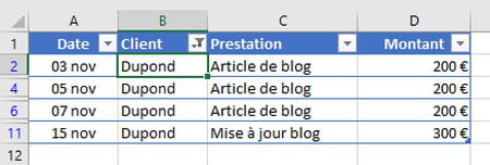
Only the lines corresponding to this customer remain displayed: you will therefore see the duplicates. The other lines are simply hidden, you can see it on the left, in our illustration, the line numbers indicate: 1, 2, 4, 6, 11 (while lines 3, 5, 7, 8, 9 , 10 are hidden).

You could add filter criteria on the other columns. For a multi-criteria search, for example to retain only the service Blog article of the customer Dupond, click, in addition, on the drop-down arrow Service to check only this caption. Alternatively, you could request that the cell contain (or not contain) text that you specify, etc.

To delete a filter on a column, click on the drop-down button then on Clear filter.

To permanently deactivate the filters and remove the small drop-down arrows: on the tab Home, click on Sort and filter, And then Filter.

How to filter data to hide duplicates in Excel?

Filters allow you to display only duplicates in a worksheet. But you can use Excel's advanced filters to, on the contrary, hide them without removing duplicate data. Note that this feature is only available in the Windows and Mac versions of Excel, and not in the web version.

In your data range, select only the column that is likely to have duplicates. Click for example on its first value and press the three keys Ctrl + Shift + Down Arrow.

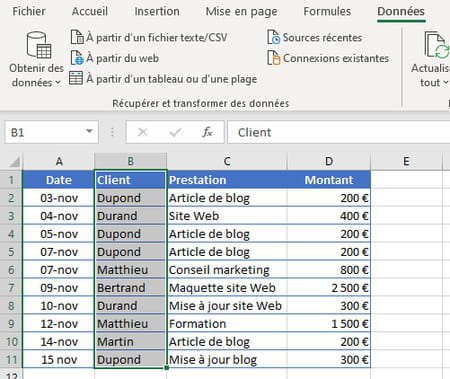
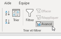
Click, at the top, on the tab Data, And then Advanced, in the Sort and filter section.

In the window Advanced filter, make sure that only the column with the duplicates is selected.

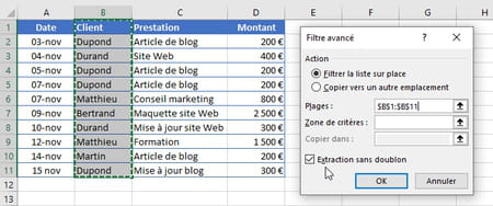
Check the box Duplicate extraction and leave the field blank Criteria area.
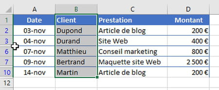
If you want Filter the list on the spot, only the first appearance of a duplicate element remains displayed, the rows of your table containing duplicates are hidden. You can see it on the left, by looking at the line numbers: in our example, we go from line 3 to line 6.

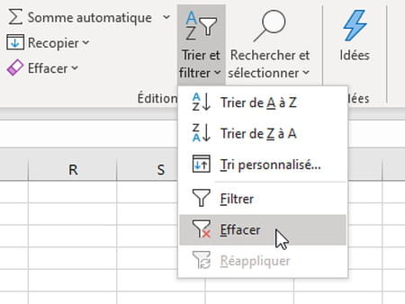
To redisplay the hidden lines, you can either: in the tab Data, click on Clear...

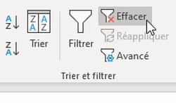
... or, in the tab Home, click on Sort and filter, And then Clear.

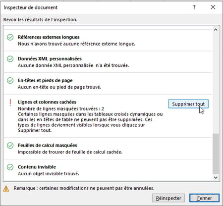
A tip on PC: if you really want to delete these hidden cells, click on the tab File> Information> button Check that there are no problems, choice Inspect the document> button Inspect… Scroll down the list of inspected problems and, in the section Hidden rows and columns, press the button Delete all. Please note, this action cannot be undone!

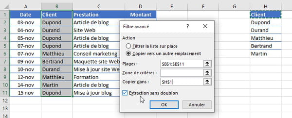
If you prefer Copy to another location (this is only possible in the active sheet), click on an empty cell, below we have chosen H1... After checking Duplicate extraction and pressed the button OK, the unique elements are copied from H1 à H6. Without touching your original table, this column could be used to calculate the amount generated by each customer, we will show you the formula below.

How to remove duplicates in Excel?

Want to permanently remove duplicates from a spreadsheet? If it is a multi-column table, the entire row of your table where the duplicate appears will be removed. If your data boils down to one column, you will get the list of unique data. Excel offers a special function for this. His method: he keeps the first element and removes all the duplicates that it then detects, without worrying about the relevance of keeping the first rather than the last, and without, for example, performing any accumulation (learn here how to accumulate duplicates). Depending on your data, a prior sorting will therefore sometimes be useful ...

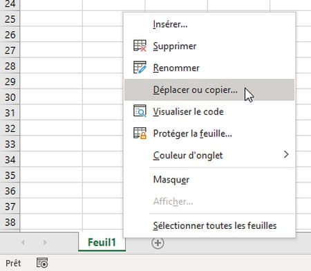
Even if it is obviously possible to cancel the action (Ctrl + Z on PC or Cmd + Z on Mac), it is best to work on a copy of your data or even duplicate the spreadsheet before performing the deletion. A little right click on the worksheet tab will help you ...

Although it is not required, it is best if your columns have a header row.
Click on a single cell, any, from your table.
In the tab Data, click on Remove duplicates.

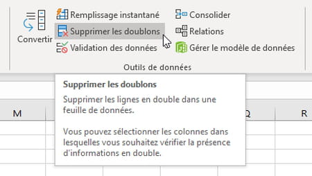
If you have transformed your data into an Excel "table" via the tab Home > Format as a table, this option Remove duplicates can also be found in the tab Table creation on PC, or Table on Mac, or Creation in Excel for the web. This tab is only visible when you select one of the table cells.
Excel selects the entire table and lists the column headers it has marked.

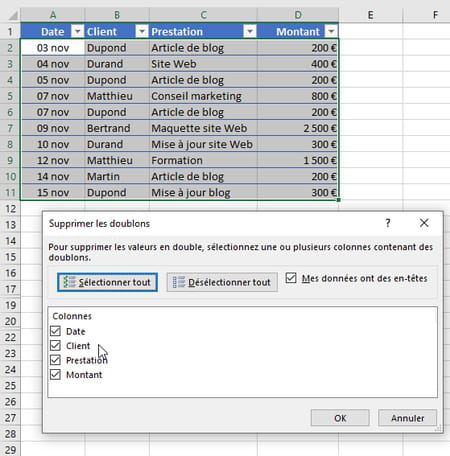
Rest assured: whether you check or uncheck such or such a box, Excel does not risk deleting a value in a column without affecting the others on the same row, which would create a shift like a badly buttoned shirt! If he has to delete a duplicate, in any case, he will delete a complete line data range (cells outside your table are not impacted).
If you leave all the column names checked, Excel will consider as duplicates only the rows where appear, in our example: both the same date, but in addition the same customer name, but also the same type of service, and finally the same amount. If any of the values differ in the rows below, they will not be considered a duplicate.
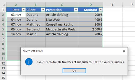
More likely, therefore, you will want to check off only certain columns. By checking for example only the column service (illustration below): each customer name will only appear once in your table (3 Dupond are deleted, 1 Durand and 1 Matthieu).

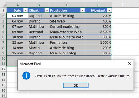
By checking for example service et benefit (illustration below): only the lines having at a time the same name et the same service are considered to be duplicates. In our example, three lines behaved like Client / Service Dupond / Blog Post values, the last two duplicate lines are removed.

Above we have considered the case where you want to remove duplicate rows directly in your table. But you could for example copy paste a single column from the table, for example copy cells B1: B11 from column Customer, to paste them in cell F1. And by asking for the deletion of duplicates in F1: F11 ...

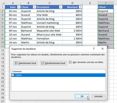
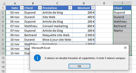
… You will get the list of your unique customers. This column can be used to calculate the turnover generated by each customer, as we will see now.

How to calculate sum of duplicates in excel sheet?

Knowing that there are duplicates is good. Delete them to keep only unique elements, why not? But most of the time, you will want to do calculations on these duplicates first, at least get the total, even if it means removing them! Here's how to go about it, depending on the method you chose to detect duplicate values.

Calculate the total of filtered values

If you have just filtered your data, a small formula will suffice to calculate the total of filtered cells, and therefore the grand total if all cells are displayed.

On a range of cells filtered via the tab Home> Sort and filter> Filter, function SOUS.TOTAL Excel allows you to calculate the sum of the displayed cells (or the average, or the number of cells, etc., depending on the parameters you specify).
On the example below, by entering in cell G1 the formula :
= SUBTOTAL (109; $ D: $ D)
to calculate the total of column D, we obtain the general total since no column is filtered here. The value 109 means: performs the sum, ignoring hidden cells.

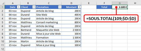
If you do not want to take into account the whole column D, but only the cells where your data is stored, the formula could be written:
= SUBTOTAL (109; D2: D11)
If we filter the column service to retain only the Smith customer, the SUBTOTAL function - which always excludes the filtered values from its calculations - tells you the total of the data displayed, therefore of the Smith customer.

Calculate the total of an Excel table

If you transformed your range of cells to an Excel table via the tab Home> Format as a table, you don't have to write a formula, Excel manages it for you.

Click in any cell of the table: a green tab Table creation on PC (or Table on Mac, or Creation in Excel for the Web) is added to the tabs already present (File, Home, Insert, etc.) at the top of the screen.
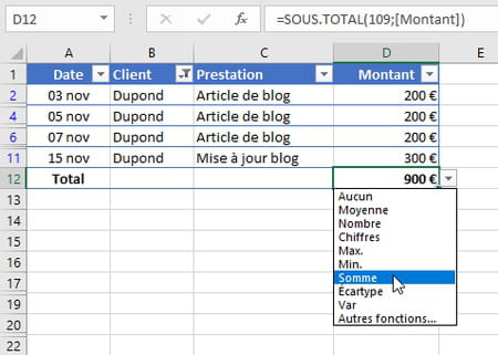
Click on this tab Table creation then, below, on Total row. Excel adds a total row at the bottom of your table, for columns that contain numbers.

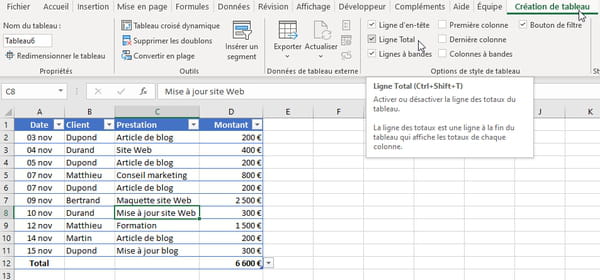
If you filter your data, the total tells you the sum of only the displayed values. A drop-down arrow lets you choose the average or another function, instead of the sum.

Calculate the total of each duplicate

Without touching your initial data, you created a column free of duplicates to keep only unique elements? If it is, for example, a list of customers, a small formula will suffice to calculate the turnover generated by each of these customers.

In our example, the column G includes the list of unique clients. The formula written in H2 allows to calculate the turnover generated by the customer registered in cell G2, therefore Dupond:
= SUM.SI ($ B: $ B; G2; $ D: $ D)

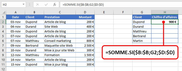
With this formula, Excel compares the contents of the cell G2 (Dupond) at each value of the column B. If there is an equivalence, it cumulates the value written on the same row, but in column D. For example, if it compares Smith to the contents of the cell B5, which also includes Dupond, it adds to its accumulation the value entered in D5.
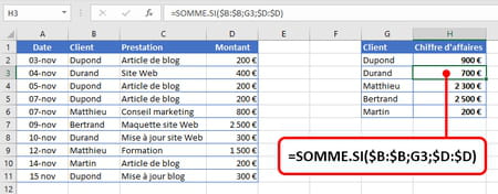
Copy this formula into the cells H3 à H6 to know the turnover generated by each customer. The formula copied into the cell H3 becomes for example:
= SUM.SI ($ B: $ B; G3; $ D: $ D)

Insert automatic subtotals in tables

Last possible solution that we offer: subtotals. Excel for Windows and for Mac (but not for the Web) can, in fact, automatically insert lines of subtotals and grand total to accumulate your data. The spreadsheet can calculate the sum, or the mean, or the min, the max, the standard deviation, etc. With some constraints to know:

Subtotals are not supported in "Excel tables". When you click on a cell in your data range, if a green tab Table creation is displayed at the top of the screen (it is called Table on Mac, and Creation in Excel for the web), you must first click below on the icon Convert to range so that you can ask Excel to insert subtotals.
As soon as you click on the icon SUBTOTAL, Excel empties its undo history. You will therefore no longer be able to cancel an old order by typing Ctrl + Z, but it is still possible to close the file and reopen it to go back to the last record in the Excel workbook. Work on a copy of your file if you are experimenting.
Inserting subtotals activates the mode Plan, which can initially impress beginners. There is no reason !

Here's how to add subtotals to your number columns.

Start by sorting your data so that the duplicates are grouped together one after the other. If it is a sort on a column, click on any value of this column (on a single cell only) then, in the tab Data, click for example on the icon AZ for a simple, ascending sort. If you need to sort on two or more columns, or specify other sorting criteria, click on the icon instead. Trier.

On the example below, our array, previously sorted on the column Date, is now sorted on the column service, in alphabetical order, by clicking on the icon AZ.

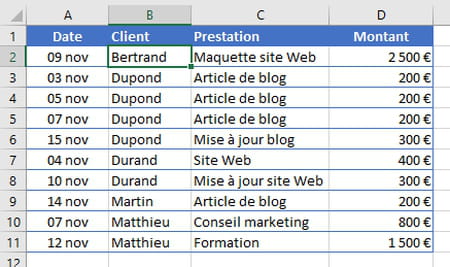
Once your data is sorted, select any cell in your table (but only one cell) and, still under the tab Data, click on the icon SUBTOTAL.
The Subtotal options window appears. Excel suggests performing a subtotal At each change of Date. Unroll this list and specify instead At each change of Client.

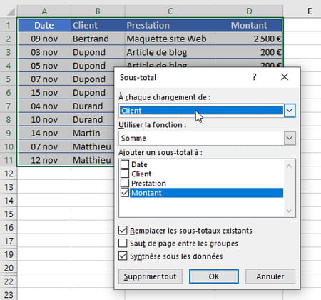
La liste Use the function indicated We Are. Click on it if you prefer another function (mean, min, max, standard deviation, number of values, etc.).
Then check the numeric items (it can be a column of invoiced sums or a column of hours indicating the duration of each service, for example) on which the accumulation must be carried out.
If you prefer the grand total row to appear at the top of the table rather than the end of the list, and each customer's subtotal to appear above rather than below their detail rows, uncheck the box Summary under the data.
Note the presence of the button Delete all, to remove the subtotal lines and deactivate the Plan world.
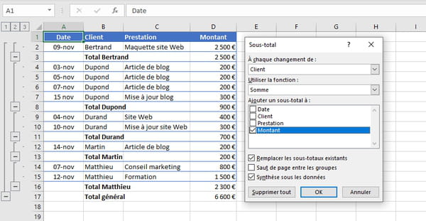
Here is our table with, for our Amount column, the subtotals in bold inserted by Excel (Total Bertrand, Total Dupond, etc.), and the Grand total at the end of the list. For your part, if your table has several columns that deserve a subtotal (columns of numbers, durations, etc.), check several.

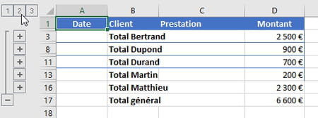
On the left, if you click on the 2 level of the plan, you only display the lines corresponding to the subtotals and the grand total.

If you perform hourly calculations and find that the hourly totals are wrong because always brought back to 24:00:00 (21h + 5h = 2h instead of 26h!), Select the cells containing your hourly data, right click on them mouse, choose Cell Format from the context menu. Under the tab Name, left click on Hour and, in the list Type, click on the format-example 37:30:55.

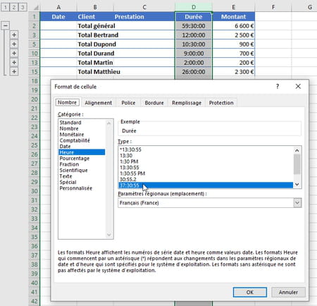
Excel now displays the correct hourly totals! Want to create a custom time format? Surround the [H] representing the hours to ask Excel to display times greater than 24 hours: [h]:mm:ss instead of h:mm:ss

How to prohibit the entry of duplicates in an Excel column?

To prevent the same value from being entered more than once in a column, all you have to do is use Excel's data validation function.

Select the entire column or range of cells where you will need to enter your data, below column B.

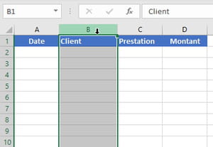
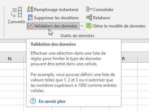
In the tab Data, click on Data validation.

In the list To allow, select custom.
In the input area Formulas, since cell B1 is currently selected, type the formula:
= NB.SI (B: B; B1) = 1

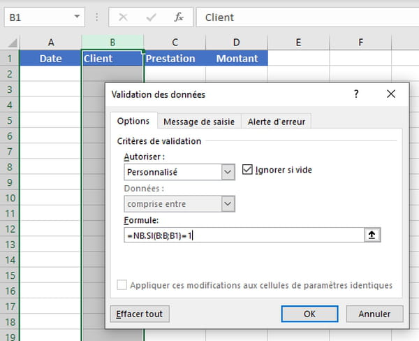
Adapt this formula: if for example cell C3 is selected, type = NB.SI (C: C; C3) = 1
In this same dialog window of Data validation, click on the tab Error alert.

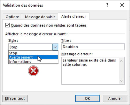
In the zone Title, enter a short message, here Duplicate.
In the zone Error message, be more explicit.
In the zone Style : the choice Stop prohibit the entry of duplicates; choices Disclaimer ou Information display your message but let the user enter a duplicate if they wish.
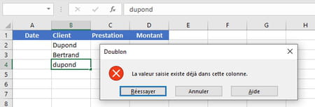
In this example, when you press the key Starter, the style Stop forbids entering Dupond twice, even in lowercase letters, and proposes to Retry.

For more information on data validation and input help, in particular using drop-down lists, see our practical sheet Create drop-down lists in Excel.

Remove duplicate Excel files: all techniques

Contents Identify duplicates in columns Filter data to display duplicates Filter data to hide duplicates Delete duplicates in Excel Calculate the sum of duplicates Prohibit the entry of ...